
Choose the model that matches the observed interval
A steady-state CO₂ estimate uses an assumed generation rate and stable indoor and outdoor concentrations to infer ventilation. A decay estimate uses the decline in CO₂ above a stable background after continuing sources are absent. They describe different operating conditions; an occupied, changing-concentration record should not be treated as a source-free decay.
Both methods need a representative, approximately well-mixed zone. A plausible number cannot establish that the air is well mixed, that occupancy and generation were stable, or that the background was appropriate. CO₂ is a tracer for the stated balance, not a complete measure of air quality or ventilation adequacy.
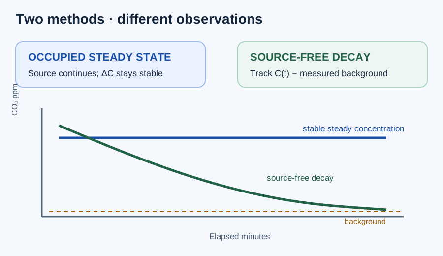
| Mode | Required condition | Inputs |
|---|---|---|
| Occupied steady state | Stable generation, population, ventilation and representative concentrations | Generation per person, occupants, indoor and outdoor ppm |
| Two-point decay | Source-free interval with stable background and operation | Initial/final ppm, actual elapsed minutes, background and room volume |
| Log-excess regression | Same source-free basis across the entire series | 3–200 increasing time/ppm rows, background and room volume |
Enter a steady-generation balance
Select Occupied steady-state generation balance. Enter justified CO₂ generation per person in L/s·person, a positive whole-number population, representative indoor steady ppm, and measured outdoor ppm. Indoor concentration must exceed outdoor concentration. The example generation of 0.005 L/s·person is illustrative; generation depends on the actual population and activity.
The concentration difference is in ppm, so multiply generation by one million when solving for air volume flow. The output includes total estimated CFM, per-person L/s, and total generation. It does not calculate the time required to reach steady state or check that the observations actually reached it.
Qoutdoor [L/s] = Gperson × N × 10⁶ / (Cindoor − Coutdoor)
Qoutdoor [CFM] = Qoutdoor [L/s] × 2.118880003
| Symbol | Meaning | Unit |
|---|---|---|
| Gperson | CO₂ generation rate for the specified activity/population | L/s·person |
| N | Occupants in the modeled condition | people |
| Cindoor, Coutdoor | Representative simultaneous steady/background concentrations | ppm |
| Qoutdoor | Flow inferred under the stated single-zone assumptions | L/s or CFM |
Enter a source-free decay interval or series
Select the two-point or regression mode. Record the interval, sensor and calibration/placement, measured stable replacement-air background, room air volume, and unchanged operating condition. Confirm a well-mixed source-free zone without an unresolved sink or interzone contribution. The calculator does not provide a gas-release procedure or exposure target.
For two points, initial and final indoor ppm must both exceed background, final must be below initial, and elapsed minutes must be positive. For regression, enter 3–200 complete rows of elapsed minutes and indoor ppm, with strictly increasing nonnegative times and each concentration above background. Nonuniform spacing is allowed. The tool neither sorts timestamps nor removes rows. Local rises remain in a series if its overall fitted log slope is negative.
The natural logarithm applies to concentration above background, not raw indoor concentration. Regression fits both slope and intercept; two-point mode does not invent regression statistics. ACH follows the negative log slope, and room volume converts it to model-equivalent CFM.
Excess concentration: E(t) = C(t) − Cbackground
Two-point ACH = (60/Δtminutes) ln[Einitial/Efinal]
Series: ln E(t) = a + bt; ACH = −60b
Model-equivalent CFM = ACH × Vroom / 60
Independent steady-state example
Use 10 people, an assumed generation of 0.005 L/s CO₂ per person, indoor 1,000 ppm, and measured background 400 ppm for this constructed case. Total generation is 0.005 × 10 = 0.05 L/s. Excess concentration is 1,000 − 400 = 600 ppm. Therefore Q = 0.05 × 1,000,000 / 600 = 83.333333 L/s, or 83.333333 × 2.118880003 = 176.573334 CFM.
The calculator displays 176.573 CFM, agreeing after rounding to three decimals. The 400 ppm value is a teaching input, not a claim about current outdoor CO₂, and 1,000 ppm is not an acceptance threshold.
Q = (0.005 × 10 × 10⁶)/(1,000 − 400) = 83.333333 L/s
83.333333 × 2.118880003 ≈ 176.573 CFM
Independent decay example and regression cross-check
Use a constructed 6,000 ft³ source-free zone with stable measured background of 400 ppm. Indoor CO₂ declines from 1,400 to 900 ppm over 10 minutes. Excess declines from 1,000 to 500 ppm. ACH = (60/10) × ln(1,000/500) = 4.158883083 h⁻¹. Model-equivalent airflow = 4.158883083 × 6,000 / 60 = 415.888308 CFM. The calculator displays 4.159 ACH and 415.888 CFM.
For a four-reading cross-check, enter 0/1,400, 10/900, 20/650, and 30/525 as minute/ppm pairs. Background-corrected excess halves every 10 minutes, so the natural-log values lie on a straight line with slope −ln(2)/10 = −0.0693147181 min⁻¹. Free-intercept regression therefore gives the same ACH. Ideal constructed R² is 1 and residuals are approximately zero; neither establishes field validity.
All displayed concentrations in this example are constructed input data. ACH and CFM use the unrounded logarithmic rate; rounding ACH first would slightly change the final CFM.
| Elapsed minutes | Indoor ppm | Excess ppm | ln(excess) |
|---|---|---|---|
| 0 | 1,400 | 1,000 | 6.907755279 |
| 10 | 900 | 500 | 6.214608098 |
| 20 | 650 | 250 | 5.521460918 |
| 30 | 525 | 125 | 4.828313737 |
Inspect assumptions and residuals before using the estimate
For a steady result, review the generation assumption and whether occupancy and concentrations were stable. For decay, review background stability, continuing sources, mixing, sensor lag, open doors, interzone exchange, and ventilation changes. Concentration differences near background are especially sensitive to errors in background and sensor readings.
The regression reports fitted concentrations, residuals, R², and a conditional ACH standard error. Its statistical error assumes independent, equal-variance log residuals. It does not include sensor calibration, serial correlation, background uncertainty, room-volume uncertainty, or model bias. A flat or rising trace that is rejected does not prove zero outdoor airflow.
A decay rate describes tracer dilution under the selected assumptions. It does not separate mechanical outdoor supply from infiltration or other paths. Particle filters and portable air cleaners generally do not remove CO₂, so their particle clean-air delivery is not measured by this decay. Use independent airflow and ventilation-method evidence for the actual engineering decision.
FAQs
Should I use steady-state or decay mode? Use steady state when generation and a stable concentration are appropriate; use decay when a source-free concentration interval is measured.
Does a CO₂ result prove ventilation compliance or safety? No. It depends on the source, mixing, occupancy, sensors, and selected model.
Can a poor regression fit be hidden by using the fitted rate? No. Review residuals and the measurement interval before using a decay estimate.
Conclusion and limits
Choose steady state or decay from the measured situation, preserve the source and mixing assumptions, and inspect fit and residuals before using the estimate.
The result is a model-based ventilation estimate, not a safety, exposure, code, or field-measurement certificate.