
A traverse has two separate jobs
A duct traverse first defines where readings will be taken; a separate calculation then converts the readings into an area-weighted average velocity and airflow. The site provides two separate tools for these jobs. The Duct Traverse Point Layout Calculator applies the listed TSI-106 Rev C, U.S. guide point fractions. The Duct Traverse Airflow Calculator reduces a set of direct-velocity readings or Pitot velocity-pressure readings. A layout is not a measured airflow, and a calculated average does not certify that the field traverse met a particular TAB procedure.
Use the project specification and the actual instrument manual to choose the method, confirm safe access, and check whether the measurement section is suitable. The layout page does not evaluate straight-run length, swirl, obstructions, probe reach, or uncertainty.
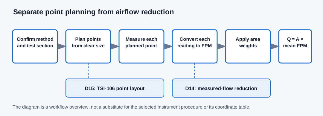
| Stage | Calculator or field action | Output |
|---|---|---|
| Plan locations | Duct Traverse Point Layout Calculator | TSI-106 point depths or grid coordinates from clear inside dimensions |
| Collect readings | Use the actual probe and field procedure | Raw velocity or velocity-pressure reading at each planned point |
| Reduce readings | Duct Traverse Airflow Calculator | Area-weighted mean velocity and actual CFM at the entered density basis |
| Compare with target | Use a compatible balancing/design record | Difference from the stated target; no automatic pass criterion |
Plan locations from the actual clear dimensions
Select round or rectangular layout and enter the finished inside dimensions after any liner. For a round duct, choose six, eight, or ten points per diameter and either two perpendicular axes or three axes 60 degrees apart. TSI-106 identifies three axes as preferred and two axes as an alternative. The calculator help follows that guide by describing six points as common at 10 inches or smaller and eight or ten points above 10 inches; confirm the job specification. The calculator’s point fractions are copied from TSI-106 Rev C, U.S. version, dated April 7, 2021; they are not a generic statement that every other TAB specification uses the same pattern.
For a rectangular duct, the implemented U.S. table selects five, six, or seven positions independently across width and height using the TSI inch thresholds: below 30 inches, 30 through 36 inches inclusive, and above 36 inches. The grid contains every combination of selected X and Y positions. It produces 25 to 49 points; a 2-by-2 grid is not part of this selected method.
Inner-wall coordinates are measured from the clear inside wall or the stated origin shown by the diagram. Outer-face marking mode adds only the offset entered by the user. It does not derive sheet thickness, insulation, drill location, tool clearance, or probe insertion hardware from nominal duct size.
- Check that the probe can physically reach each planned location without touching the wall or obstructing the reading.
- Retain the selected method, duct dimensions, point count, axis orientation, and coordinate origin with the field sheet.
- Do not replace the listed U.S. inch bands with SI thresholds or rounded coordinates from another publication.
| Dimension | Selected positions | Independent coordinate calculation |
|---|---|---|
| Width: 36 in | 6 positions | 36 × [0.061, 0.235, 0.437, 0.563, 0.765, 0.939] = [2.196, 8.460, 15.732, 20.268, 27.540, 33.804] in |
| Height: 24 in | 5 positions | 24 × [0.074, 0.288, 0.500, 0.712, 0.926] = [1.776, 6.912, 12.000, 17.088, 22.224] in |
| Complete grid | 6 × 5 = 30 points | Use every X/Y coordinate combination; origin is lower-left inner corner |
Enter the measured quantity and the field basis
After collecting the readings, select the same quantity the instrument reports. Direct-velocity mode accepts already corrected point velocities in FPM. Do not apply a Pitot coefficient or density correction again if the instrument has already applied it.
Pitot mode accepts point velocity pressures in inches of water gauge, a positive clear duct area in square feet, actual air density in lb/ft³, and one positive common velocity coefficient K that is documented for the probe and applies across the readings. The coefficient reference text is a traceability note; the calculator cannot authenticate the probe calibration. Each table row contains one reading and one positive relative sampled-area weight. Equal-area points may use weight 1. These are area weights, not confidence or statistical weights.
The form accepts up to 500 reading rows. The mean calculation rejects malformed rows rather than silently skipping them. Use a complete set that follows the applicable field method; entering fewer points does not make an incomplete traverse representative.
Direct mode: v̄ = Σ(wᵢvᵢ) / Σwᵢ
Pitot mode: vᵢ = K × 4005 × √[VPᵢ × 0.075 / ρ]
Actual airflow: Q = A × v̄
| Symbol | Meaning | Required basis |
|---|---|---|
| vᵢ | Local velocity at point i | FPM; corrected direct value or converted Pitot value |
| wᵢ | Relative area represented by point i | Positive relative weight; use 1 for equal-area sampling |
| VPᵢ | Pitot velocity pressure at point i | in. w.g.; each point is converted before averaging |
| K | Common probe velocity coefficient | Dimensionless; documented for the actual probe and range |
| ρ | Air density for Pitot conversion | lb/ft³ at the stated measurement condition |
| A | Finished clear inside duct area | ft² after liner and obstruction allowance |
| Q | Measured actual airflow | ACFM at the stated density condition, not SCFM |
Worked layout example: an 8-inch round duct
Choose round, an 8 inch clear inside diameter, six points per diameter, and three axes. The TSI-106 six-point fractions are 0.032, 0.135, 0.321, 0.679, 0.865, and 0.968. Multiply each fraction by 8 inches. The resulting depths from the negative inner-wall endpoint on each directed diameter are 0.256, 1.080, 2.568, 5.432, 6.920, and 7.744 inches. Three axes at 0, 60, and 120 degrees give 18 points. The displayed depths are rounded to three decimals; the exact fraction and entered diameter govern the coordinates.
The first point on the 0-degree axis is 0.256 inches from the negative X wall, or X = −4 + 0.256 = −3.744 inches and Y = 0 from the duct center. The layout calculator reports this point and the remaining coordinates; it does not say whether the test section or access is acceptable.
Depth = fraction × clear inside diameter; 0.032 × 8 in = 0.256 in
| Point fraction | Calculation | Depth from negative wall |
|---|---|---|
| 0.032 | 0.032 × 8 | 0.256 in |
| 0.135 | 0.135 × 8 | 1.080 in |
| 0.321 | 0.321 × 8 | 2.568 in |
| 0.679 | 0.679 × 8 | 5.432 in |
| 0.865 | 0.865 × 8 | 6.920 in |
| 0.968 | 0.968 × 8 | 7.744 in |
Worked reduction example: convert points before averaging
For an illustrative standard-Pitot calculation, use a 1 ft² clear area, density 0.075 lb/ft³, K = 1, two equal-area pressure readings of 0.01 and 0.04 in. w.g., and weights of 1. The coefficient of 1 is only a mathematical teaching value; the actual probe calibration and applicable range must be established independently.
Convert each point first: v₁ = 1 × 4005 × √(0.01 × 0.075 / 0.075) = 400.5 FPM; v₂ = 1 × 4005 × √(0.04 × 0.075 / 0.075) = 801.0 FPM. Then average the velocities: (400.5 + 801.0) / 2 = 600.75 FPM. At 1 ft², the actual airflow is 600.75 ACFM. The tool’s example reports 600.75 for both mean FPM and actual CFM at that area.
Do not average the two pressure values and take one square root. Because the square-root relation is nonlinear, that would produce a different, biased result for unequal readings. The example is not a calibration method or a measurement uncertainty statement.
v̄ = (400.5 + 801.0) / 2 = 600.75 FPM; Q = 1 ft² × 600.75 FPM = 600.75 ACFM
| Point | VP | Velocity conversion with illustrative K = 1 | Weight |
|---|---|---|---|
| 1 | 0.01 in. w.g. | 400.5 FPM | 1 |
| 2 | 0.04 in. w.g. | 801.0 FPM | 1 |
| Weighted mean | Convert individually, then average | 600.75 FPM | Σw = 2 |
| Airflow | 1 ft² × 600.75 FPM | 600.75 ACFM | Actual state |
Interpret the result and its limits
The result is an area-weighted average of the readings supplied, converted using the selected measurement mode. It is actual airflow at the entered density basis. The calculator does not convert it to SCFM, correct a changing air state, estimate instrument uncertainty, repair an unsuitable measurement location, or decide whether the flow meets a design or code criterion.
Record the measurement date, equipment operating state, duct section, probe model, calibration reference, point layout, raw readings, density basis, and any instrument correction with the result. Compare it only with a target on a compatible airflow basis and under a comparable operating condition.
| Do not | Reason | Use instead |
|---|---|---|
| Average velocity pressures before taking square roots | Pitot pressure-to-velocity conversion is nonlinear | Convert each point, then calculate the area-weighted mean velocity |
| Use centerline velocity as the cross-section average | A single point does not represent the sampled area | Collect the complete method-based traverse |
| Apply K or density correction twice | Direct mode expects corrected velocity; Pitot mode applies its stated basis | Follow the actual instrument output and correction record |
| Call the result SCFM | The result uses the entered actual density | Keep it labeled ACFM unless a separate reference-state conversion is performed |
Conclusion and limits
A defensible traverse connects a named point-location method, clear inside geometry, actual instrument readings, the correct conversion for each reading, and an area-weighted reduction. The layout calculator documents its TSI-106 Rev C U.S. fractions and three-decimal display; the airflow calculator documents direct and Pitot modes. Neither certifies compliance with AMCA, ASHRAE 111, a TAB organization procedure, or an adopted code.
Use the referenced guide and the instrument manual for the actual probe and procedure. If the project requires a different method, point count, correction, or acceptance tolerance, use that requirement explicitly rather than treating the site example as a substitute.
FAQs
Does a centerline velocity represent the duct average? No. Use the prescribed equal-area or Log-Tchebycheff layout and area weighting.
Can Pitot pressure readings be averaged before converting to velocity? No. Convert each reading using the stated density and coefficient, then average the velocities.
Does a traverse result prove the duct system is balanced? No. It is a measurement at a stated location and operating condition.
Conclusion and limits
Plan the measurement grid from the actual clear geometry, convert each reading with the correct basis, and report the resulting airflow with location and operating condition.
A traverse result is a field observation for one boundary; it does not replace balancing, pressure, leakage, or system verification.