
A pickup coefficient connects a specified signal to flow
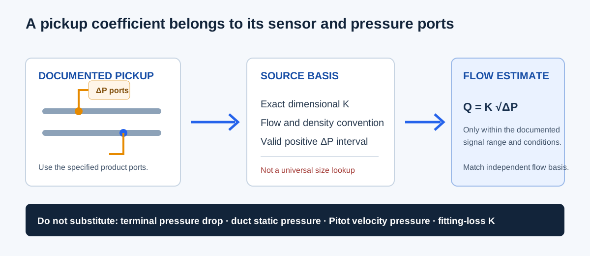
An airflow pickup K-factor is a dimensional coefficient for a particular sensor or terminal convention. It relates the differential pressure at specified pickup ports to airflow through a square-root equation. Its value depends on the product, configuration, units, flow basis, air condition, and applicable operating range. It is not a universal value for a nominal duct size or every terminal unit.
This coefficient is different from a dimensionless fitting-loss K used in pressure-loss calculations, a Pitot velocity coefficient, or an electrical transducer scale. The pickup signal is also not automatically terminal pressure drop, duct static pressure, or ordinary Pitot velocity pressure. Use the pressure from the exact ports and method named by the manufacturer.
| Quantity | Typical relationship or unit | What it describes |
|---|---|---|
| Dimensional airflow pickup coefficient | CFM/√(in. w.g.) | Product-specific flow relation for defined pickup ports |
| Fitting-loss coefficient | Dimensionless K in ΔP = K × velocity pressure | Pressure loss across a fitting or component |
| Pitot velocity coefficient | Dimensionless multiplier | Correction applied to a velocity-pressure conversion |
| Transducer scale | Electrical output per pressure | Sensor signal conversion; not itself an airflow coefficient |
Choose the mode and gather the matching inputs
The Airflow K-Factor Calculator supports three directions. In each one, the product reference and positive valid signal window must be established before interpreting the result. The confirmation records supplied assumptions; it does not validate the source or calibrate the instrument.
- Airflow from pickup signal: select the flow mode and enter the documented source coefficient K and measured positive differential pressure from the specified ports.
- Signal for a target airflow: select the pressure mode and enter the documented coefficient and positive target airflow on the source or corrected basis.
- Single-point apparent coefficient: select the coefficient mode and enter an independently measured airflow matched to a positive pickup differential at the same operating state.
- Enter the minimum and maximum valid signal from the actual pickup/instrument method. A mathematical square-root curve does not define the instrument’s usable range.
- Use the already-applicable coefficient option when its source already matches the air condition and flow convention. Select density correction only when the pickup manufacturer or method permits the model; then enter reference and actual total-air density.
| Mode | Required values | Output |
|---|---|---|
| Airflow from pickup signal | K, measured ΔP, valid signal minimum/maximum | Calculated flow at stated basis |
| Signal for target airflow | K, target flow, valid signal minimum/maximum | Required differential pressure |
| Single-point apparent coefficient | Matched independent flow and ΔP, valid signal interval | Apparent K from one observation |
| Density correction when permitted | Reference and actual total-air density | Effective coefficient for actual inlet CFM |
Equations, units, and density treatment
For a coefficient already applicable to the stated conditions, airflow Q equals K times the square root of pickup differential pressure ΔP. The inverse equation finds the pressure signal for a target airflow. The dimensional unit is CFM per square root of inches of water gauge. Since flow varies with the square root of pressure, doubling flow at the same coefficient requires four times the signal.
When the source explicitly permits the entered density correction, the calculator uses a factor equal to the square root of reference total-air density divided by actual total-air density. It multiplies the source coefficient to form an effective coefficient for actual inlet CFM. The coefficient-check mode reverses that operation to infer a source-basis apparent coefficient. Do not apply a density correction twice, and do not assume that every VAV pickup allows this correction.
Already applicable: Kₑff = Ksource; Q = Kₑff √ΔP
Permitted density model: fρ = √(ρreference / ρactual); Kₑff = Ksource fρ
Target signal: ΔP = (Q / Kₑff)²
Single-point apparent coefficient: Ksource = Qobserved / (√ΔP fρ)
| Symbol | Meaning | Unit or basis |
|---|---|---|
| Q | Airflow on the selected source or actual basis | CFM; density mode reports ACFM |
| Ksource | Documented or single-point apparent coefficient | CFM/√(in. w.g.) |
| Kₑff | Coefficient after any permitted density correction | CFM/√(in. w.g.) |
| ΔP | Differential from the specified pickup ports | in. w.g.; positive and in the documented range |
| ρreference, ρactual | Total-air mass per volume at coefficient and pickup states | lbm/ft³ |
| fρ | Permitted density multiplier | dimensionless |
Independent worked examples
Constructed example, coefficient already applicable: let K = 900 CFM/√(in. w.g.) and measured pickup differential ΔP = 0.25 in. w.g. Then √0.25 = 0.5, so Q = 900 × 0.5 = 450 CFM. With an illustrative documented signal interval of 0.01 to 1.00 in. w.g., the measured signal falls within the entered interval. The modeled endpoint flows are 90 and 900 CFM; they are not equipment capacity or control limits.
For the inverse mode, a target 450 CFM with the same K requires ΔP = (450/900)² = 0.25 in. w.g. For the apparent-coefficient mode, an independently matched 450 CFM and 0.25 in. w.g. observation gives K = 450/√0.25 = 900 CFM/√(in. w.g.). These three calculations are algebraic inverses and match the calculator’s constructed examples; none is evidence that an actual product has K = 900.
Density illustration, only if the applicable source permits it: with Ksource = 900 CFM/√(in. w.g.), ρreference = 0.075 lbm/ft³, and ρactual = 0.060 lbm/ft³, fρ = √(0.075/0.060) = 1.1180 and Kₑff = 1,006.23 CFM/√(in. w.g.). At 0.25 in. w.g., the corresponding actual flow is about 503.1 ACFM. This is a constructed mathematical illustration, not a generic VAV correction or a product recommendation.
Q = 900 × √0.25 = 450 CFM
ΔP = (450 / 900)² = 0.25 in. w.g.
Kapparent = 450 / √0.25 = 900 CFM/√(in. w.g.)
fρ = √(0.075 / 0.060) = 1.1180; Kₑff ≈ 1,006.23
| Task | Inputs | Independent result | Calculator example |
|---|---|---|---|
| Flow | K 900; ΔP 0.25 | 450 CFM | 450 CFM at stated basis |
| Target signal | Q 450; K 900 | 0.25 in. w.g. | 0.25 in. w.g. required signal |
| Apparent coefficient | Q 450; ΔP 0.25 | 900 CFM/√(in. w.g.) | 900 apparent coefficient |
| Permitted density illustration | K 900; ρref 0.075; ρactual 0.060; ΔP 0.25 | About 503.1 ACFM | Requires explicit densities; not a default example |
Interpret the answer and check the source range
The calculated flow or signal is supported only inside the positive minimum-to-maximum signal interval you entered. If a measured or required signal is outside that interval, the calculator withholds the answer; it does not clip the value or extrapolate. A signal inside the interval still does not prove sensor accuracy, installation quality, control stability, straight-run suitability, or measurement uncertainty.
A single-point apparent coefficient is one comparison at one matched condition. It does not establish repeatability, linearity, a multi-point calibration curve, or the correct controller setting. Keep the observed airflow, differential pressure, pickup ports, operating condition, source, and density treatment together. Use the product’s calibration procedure and independent evidence before changing controls.
| Check | Question to resolve | Why it matters |
|---|---|---|
| Product identity | Does K match this exact pickup/terminal configuration? | Coefficients do not transfer universally |
| Pressure ports | Was ΔP measured at the specified ports? | Static pressure, terminal loss, and pickup signal differ |
| Flow convention | Is the source coefficient for actual, standard, or another defined flow basis? | A number labeled CFM is incomplete without its convention |
| Valid signal range | Is the signal inside the source-supported window? | Formula validity does not establish instrument resolution |
| Density | Does the source permit this correction, and is it not already applied? | Prevents unsupported or duplicate correction |
| Apparent K | Was the independent airflow measured under the same state? | One unmatched point cannot identify a coefficient |
Conclusion and limits
A useful pickup calculation starts with the coefficient convention, pickup ports, flow basis, pressure interval, and air condition for the exact product. The square-root equation then connects that documented signal to flow, or solves the inverse target signal. An apparent coefficient from one observation remains a single-point comparison.
The cited Titus, Nailor, and Trane documents provide product-specific examples and show why coefficients and density treatment depend on the particular sensor or method. Their tables must not be generalized to other products. This article and calculator do not provide a universal K-factor, field calibration, controller adjustment, or code certification.
FAQs
Can a K-factor transfer between terminal models? No. It belongs to the specified pickup, ports, flow basis, and source condition.
Can I use terminal pressure drop as pickup signal pressure? No. They are different pressure boundaries.
Does a density correction apply automatically? No. Use it only when the source method permits the stated correction and it is not already applied.